Pyomo 1: largest rectangle inside a circle

Hi there, welcome! Today, we’re going to dive into a fascinating optimization problem called “Largest Rectangle Inside a Circle.” Our goal is to find the largest possible rectangle that can fit entirely inside a given circle. It may sound simple at first, but as we explore this problem, you’ll discover the intricacies and insights it offers.

To tackle this challenge, we’ll employ the power of Pyomo,  along with the non-linear solver IPopt. Together, we’ll formulate the problem, define the necessary constraints, and optimize our way to the solution.

Join us on this exciting journey as we combine mathematics, programming, and problem-solving skills to uncover the secrets of finding the largest rectangle within a circle. Let’s get started and unlock the potential of optimization with Pyomo and IPopt!

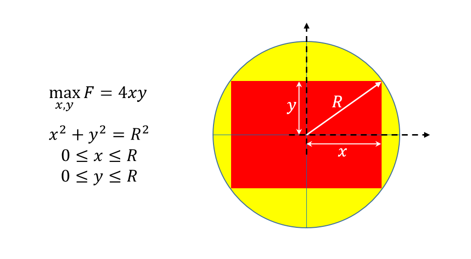
The following figure illustrates our optimization problem and one way to define it. Assuming there is no fixed value for x and y one can maximize the rectangle by maximizing its area (4xy) inside the circle.

Pyomo optimization examples biggest rectangle inside circle

The entire code can be accessed on my Github page, but here we will provide a detailed explanation of each code segment to assist you in comprehending the process of defining the problem and utilizing pyomo and its solvers to obtain a solution. I assume that you have no prior knowledge of Python programming or optimization techniques.

first, we need to import Pyomo as py or pyo (read comments carefully):

Now it is time to define the optimization problem using pyomo:


We used some objects here that need some explanation:


# import pyomo environment
import pyomo.environ as py

To get started, the initial step is to create an empty model. Pyomo provides two types of models: AbstractModel and ConcreteModel. For simplicity, let’s focus on the ConcreteModel. Defining a model in Pyomo is straightforward, you can use the following line of code. Later We will talk about the differences between these two python objects.

#define the model you can use a varaible like m or model 
m = py.ConcreteModel()

Then we defined a new variable crcR and put the value of the circle radius in it. The next step is to define a pyomo parameter and initialize it with the value of crcR.

crcR = 5
#Define parameters
m.R = py.Param(initialize=crcR)

We are now able to easily establish the variables, and there exist three significant attributes for variables. The first attribute is the bound, which determines the upper and lower limits of the variable. The second attribute is the domain, which specifies the type of variable we are dealing with. Finally, the last attribute is the initial value.

# Define variables
m.x = py.Var(bounds=(0,m.R), initialize=m.R, domain=NonNegativeReals)
m.y = py.Var(bounds=(0,m.R), initialize=m.R, domain=NonNegativeReals)

The next step involves defining constraints and an objective function, with the keyword “expr” indicating the use of an expression to define a function of variables for your constraints.

#Define constraints 
m.C1 = py.Constraint(expr = m.x**2+m.y**2==m.R**2)

The last step involves defining the objective function. You can easily express your objective using an expression and use the “sense” attribute to indicate whether you want to maximize or minimize the objective function.

#Define objective function 
m.f1 = py.Objective(expr = 4*m.x*m.y, sense = maximize)

We have fully defined the model, and now it’s time to ensure that we select the appropriate solver. If you’re interested in learning more about the solvers, you can refer to this post. However, for now, we follow a rule: if the problem is linear (where both the objective function and constraints are linear), we use GLPK as the solver. If there is at least one nonlinear term, we will use ipopt as our solver.

# Define a solver (this is not a linear program for sure) we use ipopt
solver = py.SolverFactory('ipopt')

Finally, we can solve the problem and save the results. Also you can use the object “value” to determine the value of each variable and expression(whether it is a constraint or an objective).

# Solve NLP using selected solver
results = solver.solve(m)
# print the results 
print("x= ", py.value(m.x))
print("y= ", py.value(m.y))
print("Objective value= ", py.value(m.f1))

In order to showcase the solution and demonstrate the simplicity of using matplotlib for plotting, I attempted to visually plot the results and verify them.

import numpy as np
import matplotlib.pyplot as plt

# Set the center and radius of the circle
center_x = 0
center_y = 0
radius = crcR

# Generate points along the circumference of the circle
theta = np.linspace(0, 2*np.pi, 100)
xc = center_x + radius * np.cos(theta)
yc = center_y + radius * np.sin(theta)

# Create the scatter plot
plt.plot(xc, yc, label='circle')

# Recangle corners 
# Define the coordinates of the rectangle's corners
xr = [-py.value(m.x), -py.value(m.x), py.value(m.x), py.value(m.x), -py.value(m.x)]
yr = [-py.value(m.y), py.value(m.y), py.value(m.y), -py.value(m.y), -py.value(m.y)]

plt.plot(xr, yr, label='rectangle')
plt.gca().set_aspect('equal')
plt.grid(True, linestyle='dashed')
plt.legend()

# Show the plot
plt.show()
Pyomo optimization example

Be creative and check other possibilities like if one variable be fixed what will happen to the other variable

m.x.unfix()
m.y.fix(1)
results = solver.solve(m)
# print the results 
print("x= ", py.value(m.x))
print("y= ", py.value(m.y))
print("Objective value= ", py.value(m.f1))

You can access all examples on my GitHub page.

Leave a Reply

Your email address will not be published. Required fields are marked *