
In this post, we have derived the equations of motion for an inverted pendulum cart system.
This was our first step in the process. Now, we are moving on to the next step, which is to model the system using state space and transfer function approaches.
State space representation:
Let’s start with choosing our state variables, based on the equations of motion we can choose x, \ \dot x, \ \theta , and \dot \theta as our state variables.
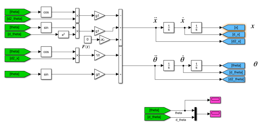
Before going any further it’s a good idea to check if our modeling is behaving as it should. for this aim open an empty model in Simulink and import the following elements:
Sum, product, cos, sin, square, integrator, gain, constant, scope, from, goto.
Connect all elements together to form the equations of motion.
If you are new to Simulink there are some tips here that you can follow for future reference. For instance, try to use “from” and “goto” blocks with a specific background color instead of making unnecessary loops (Unnecessary loops make your model debugging complicated). Additionally, it is recommended to use a consistent color, such as magenta, for all your scopes. Lastly, consider using variables and initialization files instead of hard-coding parameters in your model. To do this, right-click, select “Model properties,” go to the “Callbacks” tab, and choose “InitFcn”, write the name of your initialization file here, assume it is init_ipsc.m
init_ipscnow go to your Matlab workspace and create a new file named “init_ipsc”
edit init_ipscAdd your initialization codes and parameters and save the file:
clear
close all
clc
M = 0.5; % Cart wight in [kg]
m = 0.2; % Pendulum wight in [kg]
g = 9.8; % gravity
l = 0.3; % Pendulum length in [m]
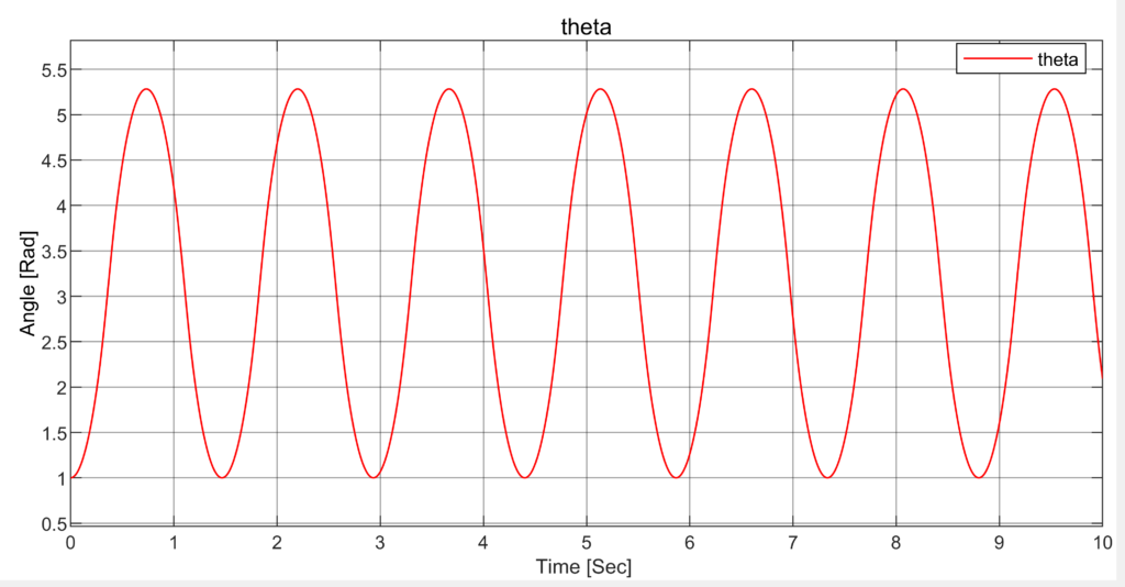
g1 = m*l/(m+M); % Gain for simplificationAlso, we may have different initial values for our states, you can assign initial values for each state using an integrator block or \frac{1}{s} , where the default value is zero. In this case, we aim to set a non-zero initial value for \theta to observe its oscillatory behavior ( \theta_0 = 1 rad ), as we do not have any friction in this system, to make sure the model is correct.
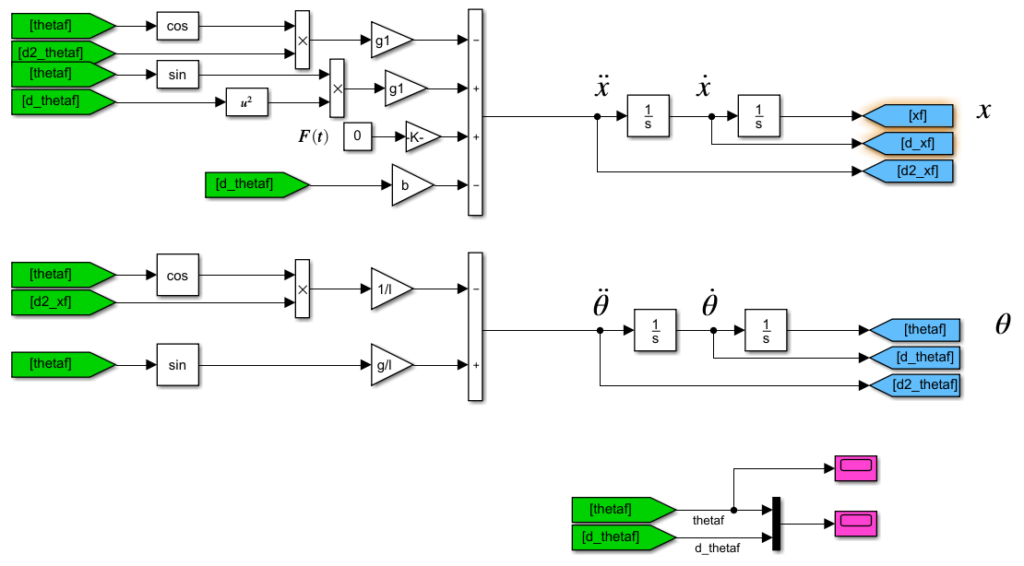
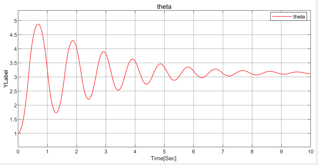
When there is friction present, the peak of oscillation gradually diminishes over time, and the angle eventually settles around the value of \pi . let us rewrite equations considering there is a friction force f_f = b \dot x and simulate the system again.
As depicted in the figure below, the pendulum’s angle initiates at 1 radian and undergoes oscillatory motion, gradually increasing before finally stabilizing at the value of \pi .
You can model your system in Simulink using a straightforward and uncomplicated method that doesn’t involve adding dozens of blocks. That method is discussed in detail in this post. However, for now, let’s continue with our simple and direct approach.
So our equations of motion behave as expected let’s linearize the system and find the state space representation.
To linearize system around \theta = 0 we can use some approximation:
With these approximations (That are valid as long as \theta is small enough ) we rewrite our set of equations:
Rewrite the given differential equations in terms of the state variables. you need some substitution and rearrangement to isolate the double differentiations from the right-hand side of the equations.
Now we have the state space representation, let’s check the Matlab code considering two outputs for the system.
M = .5;
m = 0.2;
b = 0.1;
g = 9.8;
l = 0.3;

A = [0      1              0           0;
     0     -b/M         -m*g/M         0;
     0      0              0           1;
     0   b/(l*M)       g*(M+m)/(l*M)  0];
B = [     0;
        1/M;
          0;
   -1/(l*M)];
C = [1 0 0 0;
     0 0 1 0];
D = [0;
     0];

states = {'x' 'x_dot' 'theta' 'd_theta'};
inputs = {'u'};
outputs = {'x'; 'theta'};

sys_ss = ss(A,B,C,D,'statename',states,'inputname',inputs,'outputname',outputs)
sys_ss =
A =
x x_dot theta d_theta
x 0 1 0 0
x_dot 0 -0.2 -3.92 0
theta 0 0 0 1
d_theta 0 0.6667 45.73 0
B =
u
x 0
x_dot 2
theta 0
d_theta -6.667
C =
x x_dot theta d_theta
x 1 0 0 0
theta 0 0 1 0
D =
u
x 0
theta 0