Welcome to my blog post delving into the Fascinating Field of Control. ،Today we have a fascinating opportunity to investigate the complexities of the inverted pendulum cart system. While you may not realize it, this system is found in many different places and has been used for lots of high-tech inventions, from aerospace and missile guidance systems to hoverboards, unicycles, and even rehabilitation robotics. As a classic example in the field of control systems and robotics, the IPCS offers a fascinating study of balance and control. This post’s goal is to derive the equations of motion for this system, which will help us understand its behavior and design appropriate control strategies. In this tutorial, I will provide a step-by-step guide on how to derive the equations of motion using Lagrange’s equations.
Choosing different angles for the pendulum causes confusion all the time, so I’ll do my best to solve this issue and explain that it doesn’t matter where we start measuring the angle from and we can always transfer our model to other models with other angles.
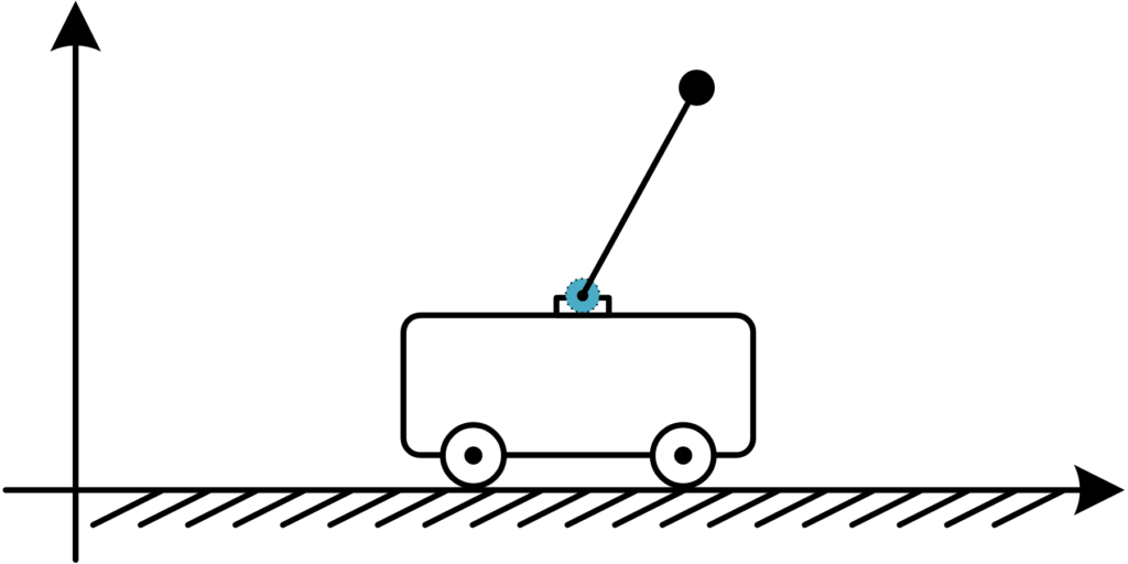
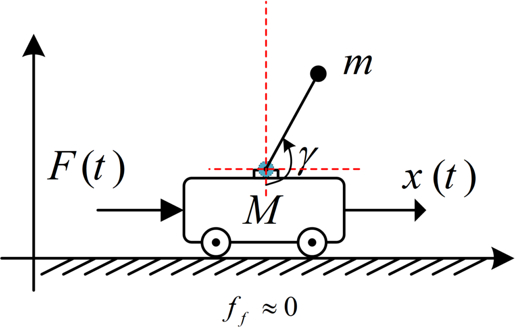
Figure 1 depicts a standard IPCS consisting of a cart that moves along a horizontal track and supports an inverted pendulum.
Figure 1: Inverted pendulum cart system
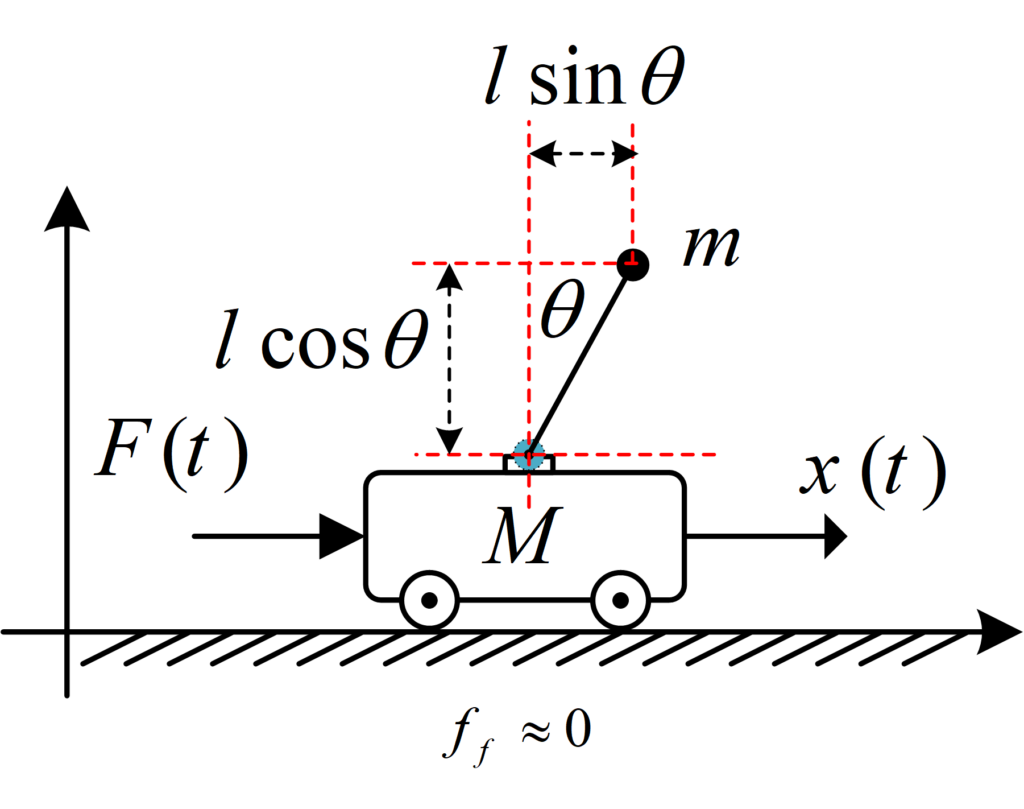
So, we have a two-degree of freedom system consisting of a pendulum with mass “m” riding on top of a cart with mass capital M. The pendulum is attached to the cart by a rigid, massless link of length “l”. To simplify things here, let’s assume a frictionless horizontal surface for the cart to move on. We’ll also consider an external force, “F(t)”, acting along the x-axis in the direction of movement. The pendulum is rotated from vertical by an amount of \theta in clockwise. Here I consider clockwise rotation as positive because it makes more sense for control purposes. For instance, if \theta is positive, we’ll need a positive force to bring the pendulum back to the vertical position, and vice versa.
Figure 2: Inverted pendulum cart system
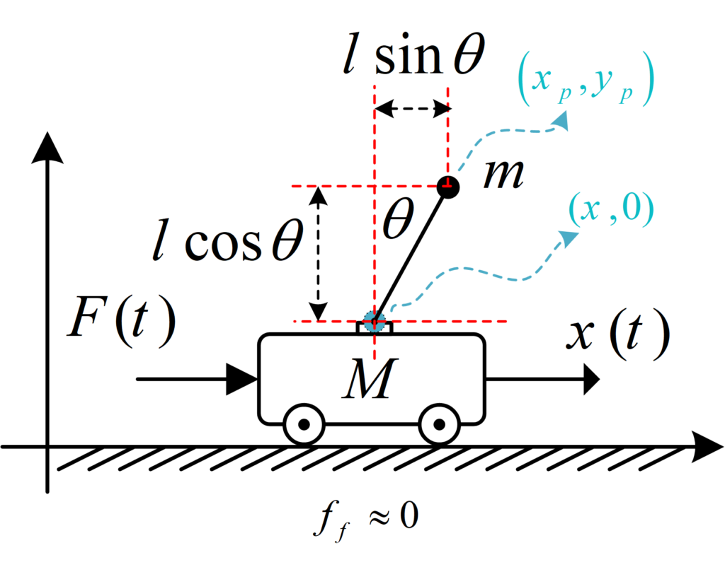
The first step is to determine the position of each mass within the system. We make the assumption that the attachment point, which connects the pendulum to the encoder, is positioned at coordinates (x, 0) and restrict the vertical movement of the cart. To determine the position of the pendulum mass, we employ kinematics, wherein we utilize the available coordinates relative to other masses for locating the mass accurately.
Figure 3: Inverted pendulum cart system kinematics
Kinematics:
{x_p} = x + l\sin \theta \\{y_p} = 0 + l\cos \theta
In order to find the velocity In each direction I can just take the time derivative of x_p\ and \ y_p so this would imply:
{{\dot x}_p} = \dot x + l\dot \theta \cos \theta \\{{\dot y}_p} = – l\dot \theta \sin \theta
ReminderWe are taking the derivatives with respect to time and not with respect to \theta which is why we are getting \dot \theta here.
In order to use Lagrange’s equations to find equations of motion we need Potential energy and Kinetic energy. For the potential energy part, since the cart is located at zero height, y_p \ = 0 , it has zero potential energy so we just need to calculate the potential energy of the pendulum mass:
Potential energy:
V = mgh = mg{y_p} = mgl\cos \theta
For Kinetic energy, it is equal to {v_i} = \frac{1}{2}{m_i}v_i^2, where m_i is the mass of ith object and v_i is it’s velocity:
To simplify matters, let’s start by understanding the concept of a generalized force denoted as Q_i . This refers to the sum of all forces acting in the direction of a specific variable. For instance, if you intend to calculate the equations of motion for the variable x you need to consider the force F(t) , In the case of a non-zero friction force represented by f_f the generalized force would be given by Q_i = F(t)-f_f .
Regarding \frac{{\partial L}}{{\partial {q_i}}} the process is straightforward. We simply need to determine the partial derivative of L with respect to all variables involved (in this case x and \theta ) However, for the remaining part of the equation \frac{d}{{dt}}\left( {\frac{{\partial L}}{{\partial {q_i}}}} \right) the understanding may not be as straightforward, so let’s make it clear as crystal by solving this part for x !
Equations of motion:
x:
First, we need to identify the components of L that contain \frac{{\partial L}}{{\partial {x}}} , so we have \frac{1}{2}\left( {m + M} \right){{\dot x}^2} and ml\dot \theta \dot x\cos \theta . Once these components have been identified, we can simply differentiate them with respect to time.
ReminderWe are taking the derivatives with respect to time and not with respect to x or \dot x which is why we are getting \ddot x and \ddot \theta here.
As there are no components that solely depend on x the second part becomes irrelevant here, also for generalized force we just have F(t) :
\left( {m + M} \right)\ddot x + ml\ddot \theta \cos \theta – ml{\dot \theta ^2}\sin \theta = F\left( t \right) \,\,\,\,\,\, \leftarrow \,\,\,\,\,\ First \ equation \ of \ motion
Let’s go for \theta part:
We have two parts that contain \dot \theta , \frac{1}{2}m{l^2}{{\dot \theta }^2} and ml\dot \theta \dot x\cos \theta , and two parts that contain \theta , ml\dot \theta \dot x\cos \theta and – mgl\cos \theta .
So let us differentiate the parts containing \dot \theta with respect to time and parts with \theta with respect to \theta
At this point we have all equations of motion we need. From here onwards you can simply follow the instructions for state space or transfer function modeling. we will discuss linearization, modeling, and simulation of IPCS in another post and check if our model is correct or not.
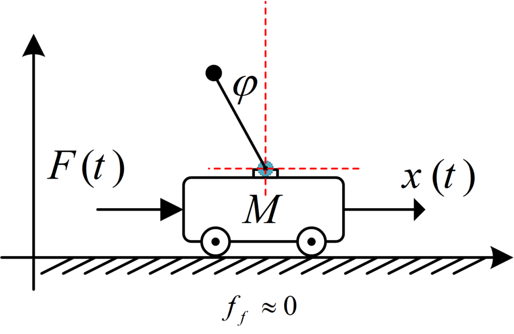
What if you choose different angle for pendulum ?Let us find out !
Suppose you have taken different angle into account for the pendulum’s rotation, and now you need to determine if your set of equations of motion are correct or not. for instance, if someone considers \varphi instead of \theta :
To find the new set of equations we just need to replace \theta with \varphi and apply all changes.